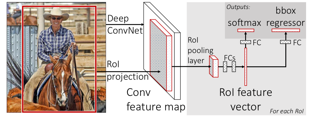
1. Motivation
R-CNN has various problems, which are
- Training is a multi-stage pipeline
- Training is expensive in space and time because features are extracted from each object proposal in each image and written to disk
- Object detection is slow
2. Architecture

Input
- Entire image
- Set of object proposals
Network
- Processes whole image with ConvNet and max pooling layers to produce a feature map
- For each object proposal, RoI pooling layer extracts fixed-length feature vector from feature map
- Each vector is fed into FC layer
Output
- Softmax probability which estimates over K object classes + “background” class
- 4 real numbers which encodes bounding-box positions for one of the K classes
2-1. RoI pooling layer
RoI pooling layer uses max pooling to convert features inside any valid RoI into a small feature map with a fixed spatial extent of H x W
2-2. Init from pre-trained networks
Use pre-trained network with transformations below
- Last max pooling layer is replaced by RoI pooling layer
- Network’s last FC layer and softmax are replaced with Fast R-CNN’s output layer
- Network is modified to take 2 data inputs
2-3 Fine-tuning: Multi-task loss
Each RoI is labeled with ground-class u and ground-truth bounding box regression target v
\[L(p,u,t^u,v)=L_{\text{cls}}(p,u)+λ[u\geq 1]L_{\text{loc}}(t^u,v)\]-
L_cls = log loss for true class u
\[L_{\text{cls}}(p,u)=-\log{p_u}\] -
L_loc = bounding box regression loss
L_loc is defined over a tuple of true bounding-box regression targets for class u and predicted tuple t^u.
\[v = (v_x, v_y, v_w, v_h)\\ t^u=(t_x^u, t_y^u, t_w^u, t_h^u)\] \[L_{\text{loc}}(t^u,v)=\sum_{i\in \{x,y,w,h\}} \text{smooth}_{L_1}(t_i^u-v_i) \\ \text{smooth}_{L_1}(x) = \begin{cases} 0.5x^2 & \text{if } |x| < 1 \\ |x| - 0.5 & \text{otherwise,} \end{cases}\]- λ : hyper-parameter that controls the balance between two losses
- [u ≥ 1] : Because for background RoIs, there is no notion of ground-truth bounding box, L_loc should be ignored
- smooth_L1 : Robust L1 loss that is less sensitive to outliers than L2 loss
2-4. Back-propagation through RoI pooling layers
\[x_i \in \mathbb{R} = \text{i-th activation input into RoI pooling layer}\\ y_{rj} = \text{layer's j-th output from r-th RoI}\]RoI pooling layer computes
\[y_{rj}=x_{i^*(r,j)} \\ i^*(r,j)=\text{argmax}_{i'\in R(r,j)}x_{i'}R(r,j)\]where i* is index set of inputs in the sub-window over which output unit y_rj max pools
Hence, backward propagation is computed with partial derivative of the loss function with respect to each input variable x_i by following the argmax switches
\[\frac{∂L}{∂x_i}=\sum_r\sum_j[i=i^*(r,j)]\frac{∂L}{∂y_{rj}}\]3. Performing Detection
Perform after Fast R-CNN is fine-tuned
- Input: image + R object proposals
- For each test RoI r, perform Forward pass → probability distribution p + predicted bounding box offsets relative to r
-
Assign detection confidence to r for each object class k using estimated probability
\[P_r(\text{class}=k\ |\ r) = p_k\] - Perform non-maximum suppression
3-1. Truncated SVD
Large FC layers are easily accelerated by compressing them with truncated SVD
\[W ≈ U\Sigma_tV^T\]Truncated SVD reduces param count from uv → t(u+v)
- FC layer can be replaced by 2 FC layers without non-linearity between them
4. Advantage
- Higher mAP
- Training is single-stage using multi-task loss
- Training can update all network layers
- No disk storage is required for feature caching