Summary
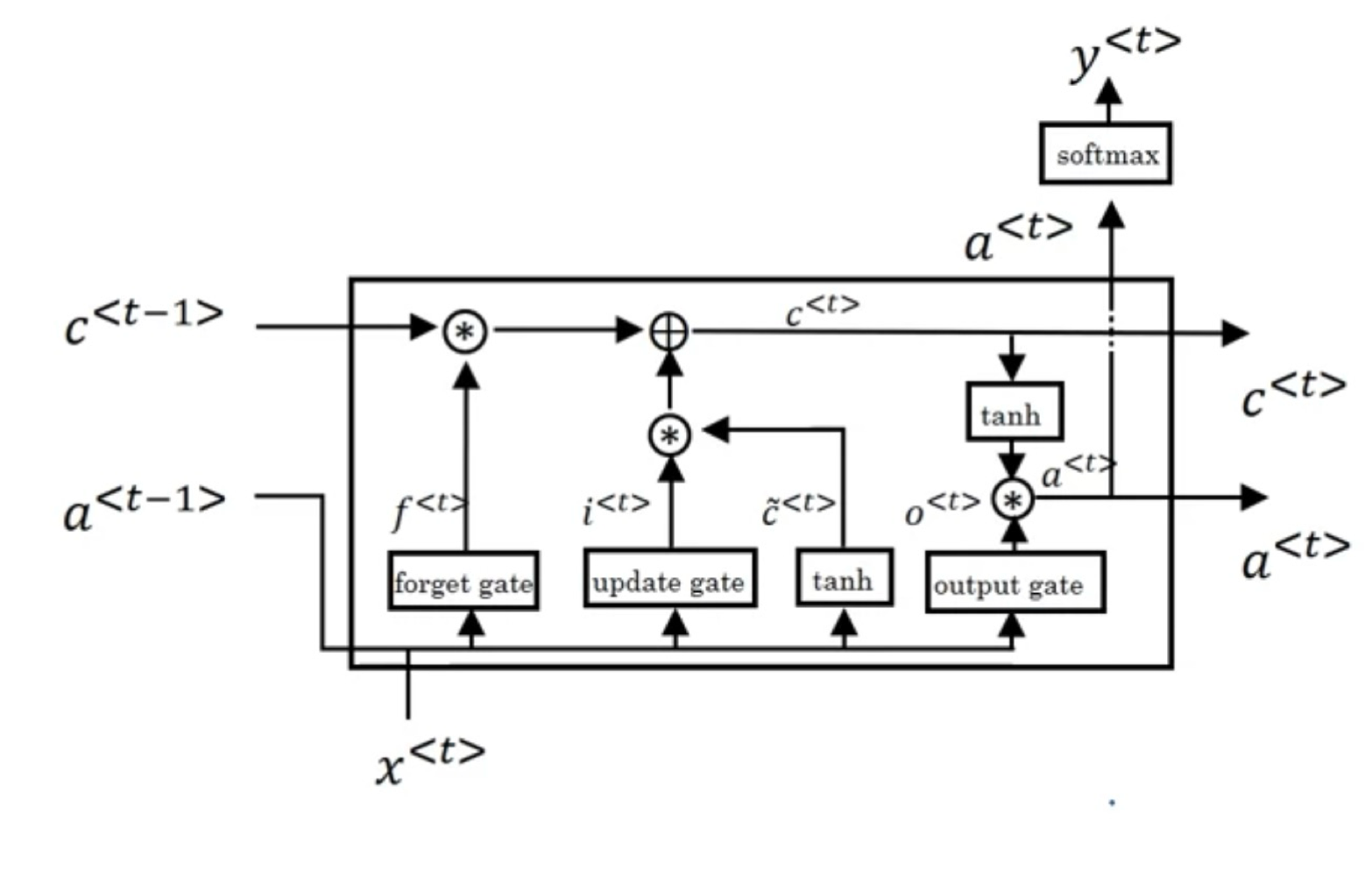
To prevent gradients from blowing up or vanishing, proposed Long-Short-Term-Memory(LSTM), which has memory cell with input gates and output gates.
In this paper, the chain of thoughts was so interesting to me.
Chain of Thoughts
- This paper begins with the explanation why gradients vanish through backpropagation.
- Introduced Naive Approach enforcing constant error flow through j, which has limitations
- Input weight conflict → weight should both store the input and protect the input → Need to control “write operations”
- Output weight conflict → weight should both access the information and protect unit from being perturbed → Need to control “read operations”
- Introduced LSTM with
- Input gates which decides when to keep or override information (write op above)
- Output gates which decides when to access memory and when to prevent (read op above)
LSTM Architecture

Why does gradient vanish?
We first start by explaining about BPTT
Back Propagation Through Time(BPTT)
Notation
\[d_k(t):\text{output unit k's target at time t}\]With label(target) y, we can measure error by using mean squared error
\[E=\frac{1}{2}(d_k(t)-y^k(t))^2\\\]We can calculate error signal by differentiating above
\[\vartheta_k(t) = f'_k(\text{net}_k(t)) (d_k(t) - y_k(t))\]where y is activation of non-input unit i with differentiable activation function f
\[y^i(t) = f_i(\text{net}_i(t))\]net_i is unit i’s current net input and w_ij is weight from j to i
\[\text{net}_i(t) = \sum_j w_{ij} y^j(t-1)\]Then, unit j’s backpropagated error signal is
\[\vartheta_j(t) = f'_j(\text{net}_j(t)) \sum_i w_{ij} \vartheta_i(t+1)\]Hochreiter’s Analysis
Assume we have fully connected net whose non-input unit indices range from 1 to n
Error occurring from unit u at time t is propagated for q time steps to unit v
\[\frac{\partial \vartheta_v(t - q)}{\partial \vartheta_u(t)} = \sum_{l_1 = 1}^{n} \cdots \sum_{l_{q-1} = 1}^{n} \prod_{m=1}^{q} f'_{l_m}(\text{net}_{l_m}(t - m)) w_{l_m l_{m-1}}\\ l_q=v,\ l_0=u\]Intuitive Explanation
-
When error blows up
\[| f'_{l_m}(\text{net}_{l_m}(t - m)) w_{l_m l_{m-1}} | > 1.0\] -
When error vanishes
\[| f'_{l_m}(\text{net}_{l_m}(t - m)) w_{l_m l_{m-1}} | < 1.0\]
If (the equation above = 1.0), error will not vanish or blow up. → Naive Approach is introduced
Naive Approach (with Limitation)
To avoid vanishing error signals, we need to achieve constant error flow through a single unit j with a single connection to itself
Because j’s local error back flow is
\[\vartheta_j(t) = f'_j(\text{net}_j(t)) \vartheta_j(t+1) w_{jj}\]We require below to enforce constant error flow through j
\[f'_j(\text{net}_j(t))w_{jj}=1.0\]Integrating(적분) the differential equation above, we can obtain
\[f_j(\text{net}_j(t))=\frac{\text{net}_j(t)}{w_{jj}}\]which means f has to be linear and unit j’s activation has to remain constant
\[y_j(t+1)=f_j(\text{net}_j(t+1))=f_j(w_{jj}y^j(t))=y^j(t)\]Limitations
In reality, unit j is not only connected to itself but also to other units
- Input weight conflict → weight should both store the input and protect the input → Need to control “write operations”
- Output weight conflict → weight should both access the information and protect unit from being perturbed → Need to control “read operations”
LSTM Architecture (overcome Limitation)
Introduced an architecture that allows constant error flow through input gate unit and output gate unit. The resulting unit is memory cell.
Notation
\[c_j:\text{memory cell}\ /\ in_j:\text{input gate}\ /\ out_j:\text{output gate}\]We have
\[y^{out_j}(t) = f_{out_j}(\text{net}_{out_j}(t)), \ y^{in_j}(t) = f_{in_j}(\text{net}_{in_j}(t))\] \[\text{net}_{out_j}(t) = \sum_u w_{out_j u} y^u(t-1) \quad \text{(output gate)}\\ \text{net}_{in_j}(t) = \sum_u w_{in_j u} y^u(t-1) \quad \text{(input gate (update gate))}\\ \text{net}_{c_j}(t) = \sum_u w_{c_j u} y^u(t-1) \quad \quad \text{(forget gate)}\]At time t, memory cell’s (LSTM’s) output is computed as
\[y^{c_j}(t)=y^{out_j}(t)h(s_{c_j}(t))\]Internal state (memory of memory cell) is computed as
\[s_{c_j}(0)=0, \ s_{c_j}(t)=s_{c_j}(t-1)+y^{in_j}(t)g(net_{c_j}(t))\]Why using gates?
To avoid input weight / output weight conflicts!
- Input gate → decides when to keep or override information in memory cell
- Output gate → decides when to access memory and when to prevent other units from being perturbed by memory.
Abuse problem and solutions
In the beginning of the learning, error reduction is possible without storing information → Network tend to abuse memory cells
Solutions
- Sequential network construction → Adds memory cell to network after error stops decreasing
- Output gate bias → Each output gate gets negative initial bias to push initial memory cell activations to 0